Introducing Dask-SearchCV

Posted on April 04, 2017

Summary

We introduce a new library for doing distributed hyperparameter optimization with Scikit-Learn estimators. We compare it to the existing Scikit-Learn implementations, and discuss when it may be useful compared to other approaches.

Introduction

Last summer I spent some time experimenting with combining dask and scikit-learn (chronicled in this series of blog posts). The library that work produced was extremely alpha, and nothing really came out of it. Recently I picked this work up again, and am happy to say that we now have something I can be happy with. This involved a few major changes:

• A sharp reduction in scope. The previous rendition tried to implement both model and data parallelism. Not being a machine-learning expert, the data parallelism was implemented in a less-than-rigorous manner. The scope is now pared back to just implementing hyperparameter searches (model parallelism), which is something we can do well.

• Optimized graph building. Turns out when people are given the option to run grid search across a cluster, they immediately want to scale up the grid size. At the cost of more complicated code, we can handle extremely large grids (e.g. 500,000 candidates now takes seconds for the graph to build, as opposed to minutes before). It should be noted that for grids this size, an active search may perform significantly better. Relevant issue: #29.

• Increased compatibility with Scikit-Learn. Now with only a few exceptions, the implementations of GridSearchCV and RandomizedSearchCV should be drop-ins for their scikit-learn counterparts.

All these changes have led to a name change (previously was dask-learn). The new library is dask-searchcv. It can be installed via conda or pip:

# conda
$ conda install dask-searchcv -c conda-forge
# pip
$ pip install dask-searchcv

In this post I'll give a brief overview of the library, and touch on when you might want to use it over other options.

What's a grid search?

Many machine learning algorithms have hyperparameters which can be tuned to improve the performance of the resulting estimator. A grid search is one way of optimizing these parameters — it works by doing a parameter sweep across a cartesian product of a subset of these parameters (the "grid"), and then choosing the best resulting estimator. Since this is fitting many independent estimators across the same set of data, it can be fairly easily parallelized.

Example using Text Classification

We'll be reproducing this example. using the newsgroups dataset from the scikit-learn docs.

Setup

First we need to load the data:

from sklearn.datasets import fetch_20newsgroups

categories = ['alt.atheism', 'talk.religion.misc']
data = fetch_20newsgroups(subset='train', categories=categories)
print("Number of samples: %d" % len(data.data))

Next, we'll build a pipeline to do the feature extraction and classification. This is composed of a CountVectorizer, a TfidfTransformer, and a SGDClassifier.

from sklearn.feature_extraction.text import CountVectorizer
from sklearn.feature_extraction.text import TfidfTransformer
from sklearn.linear_model import SGDClassifier
from sklearn.pipeline import Pipeline

pipeline = Pipeline([('vect', CountVectorizer()),
                     ('tfidf', TfidfTransformer()),
                     ('clf', SGDClassifier())])

All of these take several parameters. We'll only do a grid search across a few of them:

# Parameters of steps are set using '__' separated parameter names:
parameters = {'vect__max_df': (0.5, 0.75, 1.0),
              'vect__ngram_range': ((1, 1), (1, 2)),
              'tfidf__use_idf': (True, False),
              'tfidf__norm': ('l1', 'l2'),
              'clf__alpha': (1e-2, 1e-3, 1e-4, 1e-5),
              'clf__n_iter': (10, 50, 80),
              'clf__penalty': ('l2', 'elasticnet')}

from sklearn.model_selection import ParameterGrid
print("Number of candidates: %d" % len(ParameterGrid(parameters)))

Fitting with Scikit-Learn

In Scikit-Learn, a grid search is performed using the GridSearchCV class, and can (optionally) be automatically parallelized using joblib. Here we'll parallelize across 8 processes (the number of cores on my machine).

from sklearn.model_selection import GridSearchCV

grid_search = GridSearchCV(pipeline, parameters, n_jobs=8)

%time grid_search.fit(data.data, data.target)

Fitting with Dask-SearchCV

The implementation of GridSearchCV in Dask-SearchCV is (almost) a drop-in replacement for the Scikit-Learn version. A few lesser used parameters aren't implemented, and there are a few new parameters as well. One of these is the scheduler parameter for specifying which dask scheduler to use. By default, if the global scheduler is set then it is used, and if the global scheduler is not set then the threaded scheduler is used.

In this case, we'll use the distributed scheduler setup locally with 8 processes, each with a single thread. We choose this setup because:

• We're working with python strings instead of numpy arrays, which means that the GIL is held for some of the tasks. This means we at least want to use a couple processes to get true parallelism (which excludes the threaded scheduler).

• For most graphs, the distributed scheduler will be more efficient than the multiprocessing scheduler, as it can be smarter about moving data between workers. Since a distributed scheduler is easy to setup locally (just create a dask.distributed.Client()) there's not really a downside to using it when you want multiple processes.

Note the changes between using Scikit-Learn and Dask-SearchCV here are quite small:

from dask.distributed import Client
# Create a local cluster, and set as the default scheduler
client = Client()
client

import dask_searchcv as dcv

# Only difference here is absence of `n_jobs` parameter
dgrid_search = dcv.GridSearchCV(pipeline, parameters)

%time dgrid_search.fit(data.data, data.target)

Why is the dask version faster?

If you look at the times above, you'll note that the dask version was ~1.3X faster than the scikit-learn version. This is not because we have optimized any of the pieces of the Pipeline, or that there's a significant amount of overhead to joblib. The reason is simply that the dask version is doing less work.

Given a smaller grid

parameters = {'vect__ngram_range': [(1, 1)],
              'tfidf__norm': ['l1', 'l2'],
              'clf__alpha': [1e-3, 1e-4, 1e-5]}

and the same pipeline as above, the Scikit-Learn version looks something like (simplified):

scores = []
for ngram_range in parameters['vect__ngram_range']:
    for norm in parameters['tfidf__norm']:
        for alpha in parameters['clf__alpha']:
            vect = CountVectorizer(ngram_range=ngram_range)
            X2 = vect.fit_transform(X, y)
            tfidf = TfidfTransformer(norm=norm)
            X3 = tfidf.fit_transform(X2, y)
            clf = SGDClassifier(alpha=alpha)
            clf.fit(X3, y)
            scores.append(clf.score(X3, y))
best = choose_best_parameters(scores, parameters)

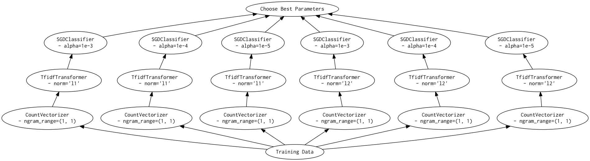
As a directed acyclic graph, this might look like:

In contrast, the dask version looks more like:

scores = []
for ngram_range in parameters['vect__ngram_range']:
    vect = CountVectorizer(ngram_range=ngram_range)
    X2 = vect.fit_transform(X, y)
    for norm in parameters['tfidf__norm']:
        tfidf = TfidfTransformer(norm=norm)
        X3 = tfidf.fit_transform(X2, y)
        for alpha in parameters['clf__alpha']:
            clf = SGDClassifier(alpha=alpha)
            clf.fit(X3, y)
            scores.append(clf.score(X3, y))
best = choose_best_parameters(scores, parameters)

As a directed acyclic graph, this might look like:

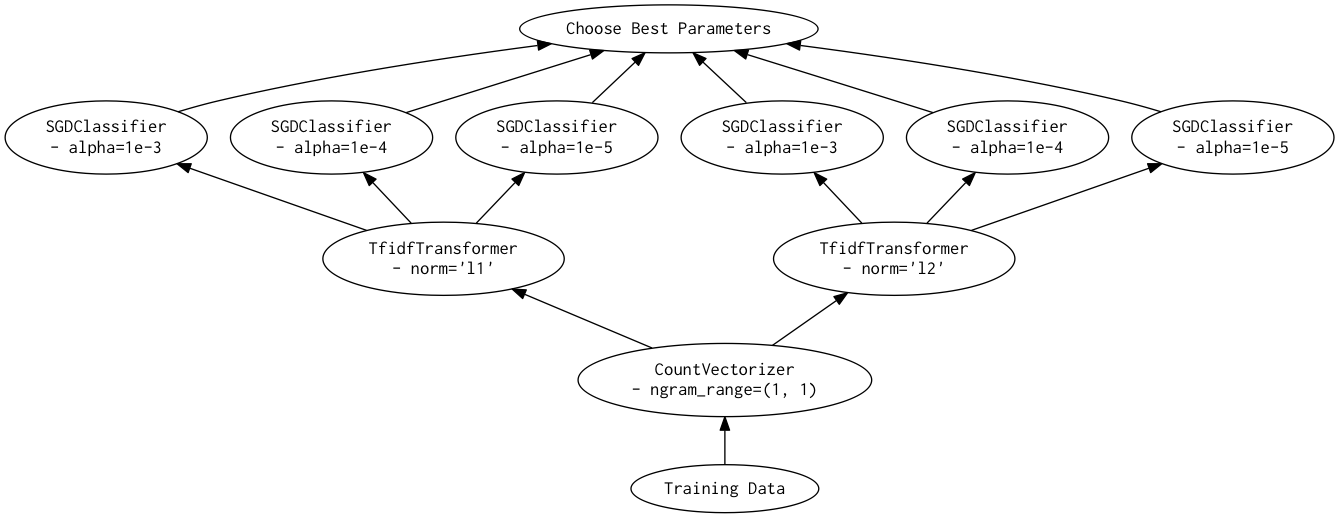
Looking closely, you can see that the Scikit-Learn version ends up fitting earlier steps in the pipeline multiple times with the same parameters and data. Due to the increased flexibility of Dask over Joblib, we're able to merge these tasks in the graph and only perform the fit step once for any parameter/data/estimator combination. For pipelines that have relatively expensive early steps, this can be a big win when performing a grid search.

Distributed Grid Search

Since Dask decouples the scheduler from the graph specification, we can easily switch from running on a single machine to running on a cluster with a quick change in scheduler. Here I've setup a cluster of 3 m4.2xlarge instances for the workers (each with 8 single-threaded processes), and another instance for the scheduler. This was easy to do with a single command using the dask-ec2 utility:

$ dask-ec2 up --keyname mykey --keypair ~/.ssh/mykey.pem --nprocs 8 --type m4.2xlarge

To switch to using the cluster instead of running locally, we just instantiate a new client, and then rerun:

client = Client('54.146.59.240:8786')
client

%time dgrid_search.fit(data.data, data.target)

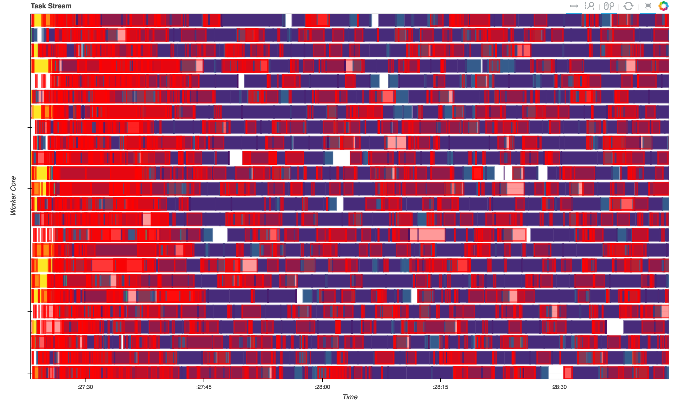
Roughly a 3x speedup, which is what we'd expect given 3x more workers. By just switching out schedulers we were able to scale our grid search out across multiple workers for increased performance.

Below you can see the diagnostic plot for this run. These show the operations that each of 24 workers were doing over time. We can see that we're keeping the cluster fairly well saturated with work (blue) and not idle time (white). There's a fair bit of serialization (red), but the values being serialized are small, so this is relatively cheap to do. Note that this plot is also a bit misleading, as the red boxes are drawn on top of the running tasks, making it look worse than it really is.

Distributed Grid Search with Joblib

For comparison, we'll also run the Scikit-Learn grid search using joblib with the dask.distributed backend. This is also only a few lines changed:

# Need to import the backend to register it
import distributed.joblib
from sklearn.externals.joblib import parallel_backend

# Use the dask.distributed backend with our current cluster
with parallel_backend('dask.distributed', '54.146.59.240:8786'):
    %time grid_search.fit(data.data, data.target)

Analysis

In this post we performed 4 different grid searches over a pipeline:

|    Library     |   Backend    | Cores |   Time   |
+----------------+--------------+-------+----------+
| Scikit-Learn   |  local       |  8    | 9min 12s |
| Dask-SearchCV  |  local       |  8    | 7min 16s |
| Scikit-Learn   |  distributed |  24   | 3min 32s |
| Dask-SearchCV  |  distributed |  24   | 2min 43s |

Looking at these numbers we can see that both the Scikit-Learn and Dask-SearchCV implementations scale as more cores are added. However, the Dask-SearchCV implementation is faster in both cases because it's able to merge redundant calls to fit and can avoid unnecessary work. For this simple pipeline this saves only a minute or two, but for more expensive transformations or larger grids the savings may be substantial.

When is this useful?

• For single estimators (no Pipeline or FeatureUnion) Dask-SearchCV performs only a small constant factor faster than using Scikit-Learn with the dask.distributed backend. The benefits of using Dask-SearchCV in these cases will be minimal.

• If the model contains meta estimators (Pipeline or FeatureUnion) then you may start seeing performance benefits, especially if early steps in the pipeline are relatively expensive.

• If the data your're fitting on is already on a cluster, then Dask-SearchCV will (currently) be more efficient, as it works nicely with remote data. You can pass dask arrays, dataframes or delayed objects to fit, and everything will work fine without having to bring the data back locally.

• If your data is too large for Scikit-Learn to work nicely, then this library won't help you. This is just for scheduling Scikit-Learn estimator fits in an intelligent way on small-medium data. It doesn't reimplement any of the algorithms found in Scikit-Learn to scale to larger datasets.

Future work

Currently we just mirror the Scikit-Learn classes GridSearchCV and RandomizedSearchCV for doing passive searches through a parameter space. While we can handle very large grids at some point switching to an active search method might be best. Something like this could be built up using the asynchronous methods in dask.distributed, and I think would be fun to work on. If you have knowledge in this domain, please weigh in on the related issue.

This work is supported by Continuum Analytics, the XDATA program, and the Data Driven Discovery Initiative from the Moore Foundation. Thanks also to Matthew Rocklin and Will Warner for feedback on drafts of this post.