Dask and Scikit-Learn -- Putting it all together
Posted on July 26, 2016
Note: This post is old, and discusses an experimental library that no longer
exists. Please see this post on dask-searchcv,
and the corresponding
documentation for the current
state of things.
This is part 3 of a series of posts discussing recent work with dask and scikit-learn.
-
In part 1 we discussed model-parallelism — fitting several models across the same data. We found that in some cases we could eliminate repeated work, resulting in improved performance of
GridSearchCVandRandomizedSearchCV. -
In part 2 we discussed patterns for data-parallelism — fitting a single model on partitioned data. We found that by implementing simple parallel patterns with a scikit-learn compatible interface we could fit models on larger datasets in a clean and standard way.
In this post we'll combine these concepts together to do distributed learning and grid search on a real dataset; namely the airline dataset. This contains information on every flight in the USA between 1987 and 2008. It's roughly 121 million rows, so it could be worked with on a single machine - we'll use it here for illustration purposes only.
I'm running this on a 4 node cluster of m3.2xlarge instances (8 cores, 30 GB
RAM each), with one worker sharing a node with the scheduler.
from distributed import Executor, progress
exc = Executor('172.31.11.71:8786', set_as_default=True)
exc
Loading the data
I've put the csv files up on S3 for faster access on the aws cluster. We can
read them into a dask dataframe using read_csv. The usecols keyword
specifies the subset of columns we want to use. We also pass in blocksize to
tell dask to partition the data into larger partitions than the default.
import dask.dataframe as dd

# Subset of the columns to use
cols = ['Year', 'Month', 'DayOfWeek', 'DepDelay',
        'CRSDepTime', 'UniqueCarrier', 'Origin', 'Dest']

# Create the dataframe
df = dd.read_csv('s3://dask-data/airline-data/*.csv',
                 usecols=cols,
                 blocksize=int(128e6),
                 storage_options=dict(anon=True))
df
Note that this hasn't done any work yet, we've just built up a graph specifying where to load the dataframe from. Before we actually compute, lets do a few more preprocessing steps:
-
Create a new column
"delayed"indicating whether a flight was delayed longer than 15 minutes or cancelled. This will be our target variable when fitting the estimator. -
Create a new column
"hour"that is just the hour value from"CRSDepTime". -
Drop both the
"DepDelay"column (using how much a flight is delayed to predict if a flight is delayed would be cheating :) ), and the"CRSDepTime"column.
These all can be done using normal pandas operations:
df = (df.drop(['DepDelay', 'CRSDepTime'], axis=1)
        .assign(hour=df.CRSDepTime.clip(upper=2399)//100,
                delayed=(df.DepDelay.fillna(16) > 15).astype('i8')))
After setting up all the preprocessing, we can call Executor.persist to fully
compute the dataframe and cache it in memory across the cluster. We do this
because it can easily fit in distributed memory, and will speed up all of the
remaining steps (I/O can be expensive).
exc.persist(df)

progress(df, notebook=False)
df
len(df) / 1e6 # Number of rows in millions
df.head()
| Year | Month | DayOfWeek | UniqueCarrier | Origin | Dest | delayed | hour | |
|---|---|---|---|---|---|---|---|---|
| 0 | 1987 | 10 | 3 | PS | SAN | SFO | 0 | 7 |
| 1 | 1987 | 10 | 4 | PS | SAN | SFO | 0 | 7 |
| 2 | 1987 | 10 | 6 | PS | SAN | SFO | 0 | 7 |
| 3 | 1987 | 10 | 7 | PS | SAN | SFO | 0 | 7 |
| 4 | 1987 | 10 | 1 | PS | SAN | SFO | 1 | 7 |
So we have roughly 121 million rows, each with 8 columns each. Looking at the columns you can see that each variable is categorical in nature, which will be important later on.
Exploratory Plotting
Now that we have the data loaded into memory on the cluster, most dataframe computations will run much faster. Lets do some exploratory plotting to see the relationship between certain features and our target variable.
# Define some aggregations to plot
aggregations = (df.groupby('Year').delayed.mean(),
                df.groupby('Month').delayed.mean(),
                df.groupby('hour').delayed.mean(),
                df.groupby('UniqueCarrier').delayed.mean().nlargest(15))

# Compute them all in a single pass over the data
(delayed_by_year,
delayed_by_month,
delayed_by_hour,
delayed_by_carrier) = dask.compute(*aggregations)
Plotting these series with bokeh gives:
The hour one is especially interesting, as it shows an increase in frequency of delays over the course of each day. This is possibly due to a cascading effect, as earlier delayed flights cause problems for later flights waiting on the plane/gate.
Extract Features
As we saw above, all of our columns are categorical in nature. To make best use of these, we need to "one-hot encode" our target variables. Scikit-learn provides a builtin class for doing this, but it doesn't play as well with dataframe inputs. Instead of making a new class, we can do the same operation using some simple functions and the dask delayed interface.
Here we define a function one_hot_encode to transform a given
pandas.DataFrame into a sparse matrix, given a mapping of categories for each
column. We've decorated the function with dask.delayed, which makes the
function return a lazy object instead of computing immediately.
import pandas as pd
import numpy as np
from dask import delayed
from scipy import sparse

def one_hot_encode_series(s, categories, dtype='f8'):
    """Transform a pandas.Series into a sparse matrix by one-hot-encoding
    for the given `categories`"""
    cat = pd.Categorical(s, np.asarray(categories))
    codes = cat.codes
    n_features = len(cat.categories)
    n_samples = codes.size
    mask = codes != -1
    if np.any(~mask):
        raise ValueError("unknown categorical features present %s "
                        "during transform." % np.unique(s[~mask]))
    row_indices = np.arange(n_samples, dtype=np.int32)
    col_indices = codes
    data = np.ones(row_indices.size)
    return sparse.coo_matrix((data, (row_indices, col_indices)),
                            shape=(n_samples, n_features),
                            dtype=dtype).tocsr()


@delayed(pure=True)
def one_hot_encode(df, categories, dtype='f8'):
    """One-hot-encode a pandas.DataFrame.

    Parameters
    ----------
    df : pandas.DataFrame
    categories : dict
        A mapping of column name to an sequence of categories for the column.
    dtype : str, optional
        The dtype of the output array. Default is 'float64'.
    """
    arrs = [one_hot_encode_series(df[col], cats, dtype=dtype)
            for col, cats in sorted(categories.items())]
    return sparse.hstack(arrs).tocsr()
To use this function, we need to get a dict mapping column names to their
categorical values. This isn't ideal, as it requires a complete pass over the
data before transformation. Since the data is already in memory though, this is
fairly quick to do:
# Extract categories for each feature
categories = dict(Year=np.arange(1987, 2009),
                  Month=np.arange(1, 13),
                  DayOfWeek=np.arange(1, 8),
                  hour=np.arange(24),
                  UniqueCarrier=df.UniqueCarrier.unique(),
                  Origin=df.Origin.unique(),
                  Dest=df.Dest.unique())

# Compute all the categories in one pass
categories = delayed(categories).compute()
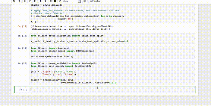
Finally, we can build up our feature and target matrices, as two
dklearn.matrix.Matrix objects.
import dklearn.matrix as dm

# Convert the series `delayed` into a `Matrix`
y = dm.from_series(df.delayed)

# `to_delayed` returns a list of `dask.Delayed` objects, each representing
# one partition in the total `dask.dataframe`
chunks = df.to_delayed()

# Apply `one_hot_encode` to each chunk, and then convert all the
# chunks into a `Matrix`
X = dm.from_delayed([one_hot_encode(x, categories) for x in chunks],
                    dtype='f8')
X, y
Extract train-test splits
Now that we have our feature and target matrices, we're almost ready to start
training an estimator. The last thing we need to do is hold back some of the
data for testing later on. To do that, we can use the train_test_split
function, which mirrors the scikit-learn function of the same
name.
We'll hold back 20% of the rows:
from dklearn.cross_validation import train_test_split

X_train, X_test, y_train, y_test = train_test_split(X, y, test_size=0.2)
Create an estimator
As discussed in the previous post,
dask-learn contains several parallelization patterns for wrapping scikit-learn
estimators. These make it easy to use with any estimator that matches the
scikit-learn standard interface. Here we'll wrap a SGDClassifier with the
Averaged wrapper. This will fit the classifier on each partition of the data,
and then average the resulting coefficients to produce a final estimator.
from dklearn import Averaged
from sklearn.linear_model import SGDClassifier

est = Averaged(SGDClassifier())
Distributed grid search
The SGDClassifier also takes several hyperparameters, we'll do a grid search
across a few of them to try and pick the best combination. Note that the
dask-learn version of GridSearchCV mirrors the interface of the scikit-learn
equivalent. We'll also pass in an instance of RandomSplit to use for
cross-validation, instead of the default KFold. We do this because the
samples are ordered approximately chronologically, and KFold would result in
training data with potentially missing years.
from dklearn.cross_validation import RandomSplit
from dklearn.grid_search import GridSearchCV

grid = {'alpha': [0.0001, 0.001],
        'loss': ['log', 'hinge']}

search = GridSearchCV(est, grid,
                      cv=RandomSplit(n_iter=3, test_size=0.2))
Finally we can call fit and perform the grid search. As discussed in In part
1, GridSearchCV isn't lazy due to some
complications with the scikit-learn api, so this call to fit runs
immediately.
search.fit(X_train, y_train)
What's happening here is:
- An estimator is created for each parameter combination and test-train set
- Each estimator is then fit on its corresponding set of training data (using
the
Averagedparallelization pattern) - Each estimator is then scored on its corresponding set of testing data
- The best set of parameters will then be chosen based on these scores
- Finally, a new estimator is then fit on all of the data, using the best parameters
Note that this is all run in parallel, distributed across the cluster. Thanks to the slick web interface, you can watch it compute. This takes a couple minutes, here's a gif of just the start:
Once all the computation is done, we can see the best score and parameters by
checking the best_score_ and best_params_ attributes (continuing to mirror
the scikit-learn interface):
search.best_score_
search.best_params_
So we got ~83% accuracy on predicting if a flight was delayed based on these
features. The best estimator (after refitting on all of the training data) is
stored in the best_estimator_ attribute:
search.best_estimator_
Scoring the model
To evaluate our model, we can check its performance on the testing data we held
out originally. This illustrates an issue with the current design; both
predict and many of the score functions are parallelizable, but since we
don't know which one a given estimator uses in its score method, we can't
dispatch to a parallel implementation easily. For now, we can call predict
(which we can parallelize), and then compute the score directly using the
accuracy_score function (the default score for classifiers).
from sklearn.metrics import accuracy_score

# Call `predict` in parallel on the testing data
y_pred = search.predict(X_test)

# Compute the actual and predicted targets
actual, predicted = dask.compute(y_test, y_pred)

# Score locally
accuracy_score(actual, predicted)
So the overall accuracy score is ~83%, roughly the same as the best score
from GridSearchCV above. This may sound good, but it's actually equivalent to
the strategy of predicting that no flights are delayed (roughly 83% of all
flights leave on time).
# Compute the fraction of flights that aren't delayed.
s = df.delayed.value_counts().compute()
s[0].astype('f8') / s.sum()
I'm sure there is a better way to fit this data (I'm not a machine learning expert). However, the point of this blogpost was to show how to use dask to create these workflows, and I hope I was successful in that at least.
What worked well
-
Combining both model-parallelism (
GridSearchCV) and data-parallelism (Averaged) worked fine in a familiar interface. It's nice when abstractions played well together. -
Operations (such as one-hot encoding) that aren't part of the built-in dask api were expressed using
dask.delayedand some simple functions. This is nice from a user perspective, as it makes it easy to add things unique to your needs. -
A full analysis workflow was done on a cluster using familiar python interfaces. Except for a few
computecalls here and there, everything should hopefully look like familiarpandasandscikit-learncode. Note that by selecting a different scheduler this could be done locally on a single machine as well. -
The library demoed here is fairly short and easily maintainable. Only naive approaches have been implemented so far, but for some things the naive approaches may work well.
What could be better
-
Since scikit-learn estimators don't expose which scoring function they use in their
scoremethod,some_dask_estimator.scoremust pull all the the data to score onto one worker to score it. For smaller datasets this is fine, but for larger datasets this serialization becomes more costly.
One thought would be to infer the scoring function from the type of estimator (e.g. use `accuracy_score` for classifiers, `r2_score` for regressors, etc...). Dask versions of each could then be implemented, which would be *much* more efficient. This wouldn't work well with estimators that didn't use the defaults though.
-
As discussed in part 1,
GridSearchCVisn't lazy (due to the need to support therefitkeyword), while the rest of the library is. Sometimes this is nice, as it allows it to be a drop-in for the scikit-learn class. I'd still like to find a way to remove this disconnect, but haven't found a solution I'm happy with.
Help
I am not a machine learning expert. Is any of this useful? Do you have suggestions for improvements (or better yet PRs for improvements :))? Please feel free to reach out in the comments below, or on github.
This work is supported by Continuum Analytics and the XDATA program as part of the Blaze Project.