Dask and Scikit-Learn -- Data Parallelism

Posted on July 19, 2016

Note: This post is old, and discusses an experimental library that no longer exists. Please see this post on dask-searchcv, and the corresponding documentation for the current state of things.

This is part 2 of a series of posts discussing recent work with dask and scikit-learn. In the last post we discussed model-parallelism — fitting several models across the same data. In this post we'll look into simple patterns for data-parallelism, which will allow fitting a single model on larger datasets.

Scaling scikit-learn

Scikit-learn contains several tools for working with large datasets. The best way to learn about them is to check out the excellent documentation. In short, scikit-learn's approach needs three things:

1. A way to incrementally load data
2. A way to efficiently extract features (such as HashingVectorizer and FeatureHasher)
3. An incremental learning algorithm (estimators that implement partial_fit)

Applied together these allow scikit-learn to do out-of-core learning (working with data that doesn't fit in RAM). This works well in practice, but does present a few issues:

• Incremental learning is an inherently serial operation — the samples are streamed through the estimator updating the coefficients incrementally. Often some of the preprocessing/feature-extraction steps can be parallelized, something scikit-learn doesn't make easy to do.

• There's a disconnect between in memory estimators, which can be used with GridSearchCV, and incrememental estimators which can't. If you want to optimize hyperparameters when using partial_fit you currently have to implement that part yourself.

• There are other methods of dealing with larger datasets. One common method is model averaging, where the same model is fit on many partitions, and the resulting coefficients are averaged together at the end. This is presented in a few scikit-learn presentations, but not implemented in a builtin way anywhere (yet).

To demonstrate dask-learn's approach to solving these issues, we'll reproduce this text classification example from the scikit-learn docs.

Out-of-core classification of text documents using dask-learn

This example uses the Reuters-21578 collection, as taken from the UCI ML repository. This is a collection of documents taken from the Reuters newswire in 1987. Each document is labeled with a category describing its content (e.g. "acq").

Preprocessing

Following the scikit-learn example, we'll copy-paste in their subclass of HTMLParser. This is used for parsing the the .sgm files and yielding them one at a time.

import re

from sklearn.externals.six.moves import html_parser
from sklearn.externals.six.moves import urllib

class ReutersParser(html_parser.HTMLParser):
    """Utility class to parse a SGML file and yield documents one at a time."""

    def __init__(self, encoding='latin-1'):
        html_parser.HTMLParser.__init__(self)
        self._reset()
        self.encoding = encoding

    def handle_starttag(self, tag, attrs):
        method = 'start_' + tag
        getattr(self, method, lambda x: None)(attrs)

    def handle_endtag(self, tag):
        method = 'end_' + tag
        getattr(self, method, lambda: None)()

    def _reset(self):
        self.in_title = 0
        self.in_body = 0
        self.in_topics = 0
        self.in_topic_d = 0
        self.title = ""
        self.body = ""
        self.topics = []
        self.topic_d = ""

    def parse(self, fd):
        self.docs = []
        for chunk in fd:
            self.feed(chunk.decode(self.encoding))
            for doc in self.docs:
                yield doc
            self.docs = []
        self.close()

    def handle_data(self, data):
        if self.in_body:
            self.body += data
        elif self.in_title:
            self.title += data
        elif self.in_topic_d:
            self.topic_d += data

    def start_reuters(self, attributes):
        pass

    def end_reuters(self):
        self.body = re.sub(r'\s+', r' ', self.body)
        self.docs.append({'title': self.title,
                        'body': self.body,
                        'topics': self.topics})
        self._reset()

    def start_title(self, attributes):
        self.in_title = 1

    def end_title(self):
        self.in_title = 0

    def start_body(self, attributes):
        self.in_body = 1

    def end_body(self):
        self.in_body = 0

    def start_topics(self, attributes):
        self.in_topics = 1

    def end_topics(self):
        self.in_topics = 0

    def start_d(self, attributes):
        self.in_topic_d = 1

    def end_d(self):
        self.in_topic_d = 0
        self.topics.append(self.topic_d)
        self.topic_d = ""

Using that parser, we can create a few preprocessing functions for extracting features and targets. We'll then apply these functions to each file/document using the dask.bag interface. At the end of this process we'll have a dask.bag.Bag containing the title and body of each document as text — this will be our feature matrix. We'll also have a dklearn.matrix.Matrix of booleans indicating whether the document is labeled with the "acq" topic — this will be our target matrix. We'll then learn a binary classification problem to determine from the document text whether the document is in the "acq" class.

import os
from glob import glob
import numpy as np

import dask.bag as db
import dklearn.matrix as dm


def file_to_documents(filename):
    """Given a filename, yield documents"""
    for doc in ReutersParser().parse(open(filename, 'rb')):
        yield doc


def remove_empty_topics(docs):
    """Remove all docs that don't have a topic"""
    return [doc for doc in docs if doc['topics']]


def documents_to_X_text(docs):
    """Extract the text to use as features"""
    return [u'{title}\n\n{body}'.format(**doc) for doc in docs]


def documents_to_y(docs, pos_class='acq'):
    """Create an array indicating whether ``pos_class`` is in the
    topics for each document."""
    return np.array([pos_class in doc['topics'] for doc in docs], dtype='i1')


files = glob(os.path.join("reuters", "*.sgm"))
docs = (db.from_sequence(files)
          .map(file_to_documents)
          .map(remove_empty_topics))
X_text = docs.map(documents_to_X_text).concat()
y = dm.from_bag(docs.map(documents_to_y), dtype='i1')

Extract train-test splits

To validate our fit estimators, we'll need to hold back a sample of data to use for testing. To do that, we can use the train_test_split function, which mirrors the scikit-learn function of the same name. We'll hold back 20% of the data to use as a test set.

from dklearn.cross_validation import train_test_split

X_train, X_test, y_train, y_test = train_test_split(X_text, y, test_size=0.2)

Feature Extraction

We can't train directly on the text data, we first need to extract it out into a matrix of features. Continuing to mirror the scikit-learn example, we'll use a HashingVectorizer. This is a stateless transformer that maps tokens to integers using a hash function, and results in a sparse matrix of occurrence counts for each token. Since it's stateless it works well with out-of-core or streaming data, and the transform can be trivially mapped across all partitions. As a dask graph, this looks something like:

To do this mapping automatically, we've implemented a simple wrapper in dask-learn.

from dklearn.feature_extraction import HashingVectorizer

vectorizer = HashingVectorizer(decode_error='ignore',
                               n_features=2**18,
                               non_negative=True)

Parallelization patterns

Dask-learn contains several parallelization patterns for wrapping scikit-learn estimators. Here we'll create a Pipeline for each pattern, which we will later fit.

Chained

Chained is for use with estimators that implement the partial_fit method, and implements "partial_fit chaining". When the Chained.fit method is called, a graph is created that calls partial_fit iteratively on each chunk. As a dask graph, this looks something like:

We'll create a Pipeline that first transforms the input using the HashingVectorizer created above, and then follows it with a SGDClassifier wrapped with Chained.

from dklearn import Chained, Pipeline
from sklearn.linear_model import SGDClassifier

pipe1 = Pipeline([('vect', vectorizer),
                  ('sgd', Chained(SGDClassifier()))])
pipe1

Averaged

Averaged fits the same estimator on each chunk in parallel, and then averages the coefficients together at the end. This is a simple way to deal with larger data, and is discussed in more detail in this notebook from Olivier Grisel. As a dask graph, this looks something like:

We'll create a Pipeline as before, but this time fitting a LogisticRegression wrapped with Averaged.

from dklearn import Averaged
from sklearn.linear_model import LogisticRegression

pipe2 = Pipeline([('vect', vectorizer),
                  ('logistic', Averaged(LogisticRegression()))])
pipe2

A closer look at dask-learn estimators

It should be noted that the estimators from dask-learn created above (Chained, Averaged, Pipeline, etc...) are actual scikit-learn estimators, all deriving from the same sklearn.base.BaseEstimator class. They implement many of the common scikit-learn methods, work with sklearn.clone, and repr the same. However, all operations on them are lazy and pure. This means two things:

• Methods such as fit and set_params return a new estimator rather than mutating the estimator in place. This means that you need to do fit_est = est.fit(X, y) instead of est.fit(X, y).

• With a few exceptions (get_params, and __getattr__), all operations on the estimators are done lazily, building a dask graph behind the scenes. This means that to actually perform the fit/predict/score/etc... you need to call the compute method. This matches the same interface as the main dask collections (array, bag, dataframe, etc...).

These design decisions were made to make the code easier to reason about — trying to determine the result of lazy-mutable operations proved to be quite tricky. A benefit of the laziness is that multiple estimators can be fit at the same time sharing intermediates (as show in the previous post).

Fitting and scoring the estimators

Here we'll fit and score both estimators. Remember this is all done lazily, so no actual work will be done until we call compute.

fit1 = pipe1.fit(X_train, y_train, sgd__classes=[0, 1])
score1 = fit1.score(X_test, y_test)

fit2 = pipe2.fit(X_train, y_train)
score2 = fit2.score(X_test, y_test)

Note that the chained pipeline received a classes keyword to fit. This is because partial_fit requires the keyword on the first call. If it wasn't provided, the classes would be determined automatically, but this is less efficient. The Averaged estimator doesn't have this restriction.

To do the actual fitting, we'll pass both the fit estimators and scores to dask.compute. This will merge all the graphs together, allowing intermediates to be shared. This entire graph contains:

• All preprocessing steps
• Train-test splitting
• Both pipeline fits (Averaged and Chained)
• Estimator scoring

We'll also use the profiling functionality provided in dask.diagnostics to measure performance.

from dask.diagnostics import ResourceProfiler, Profiler, ProgressBar, visualize
from dask.multiprocessing import get as mp_get
from dask import compute

with ResourceProfiler(0.5) as rprof, Profiler() as prof, ProgressBar():
    fit1, fit2, score1, score2 = compute(fit1, fit2, score1, score2,
                                         get=mp_get, num_workers=4)

score1

score2

From these scores, it seems that the Chained(SGDClassifier()) pipeline performs better for this text classification problem. Now let's look at the profile plot:

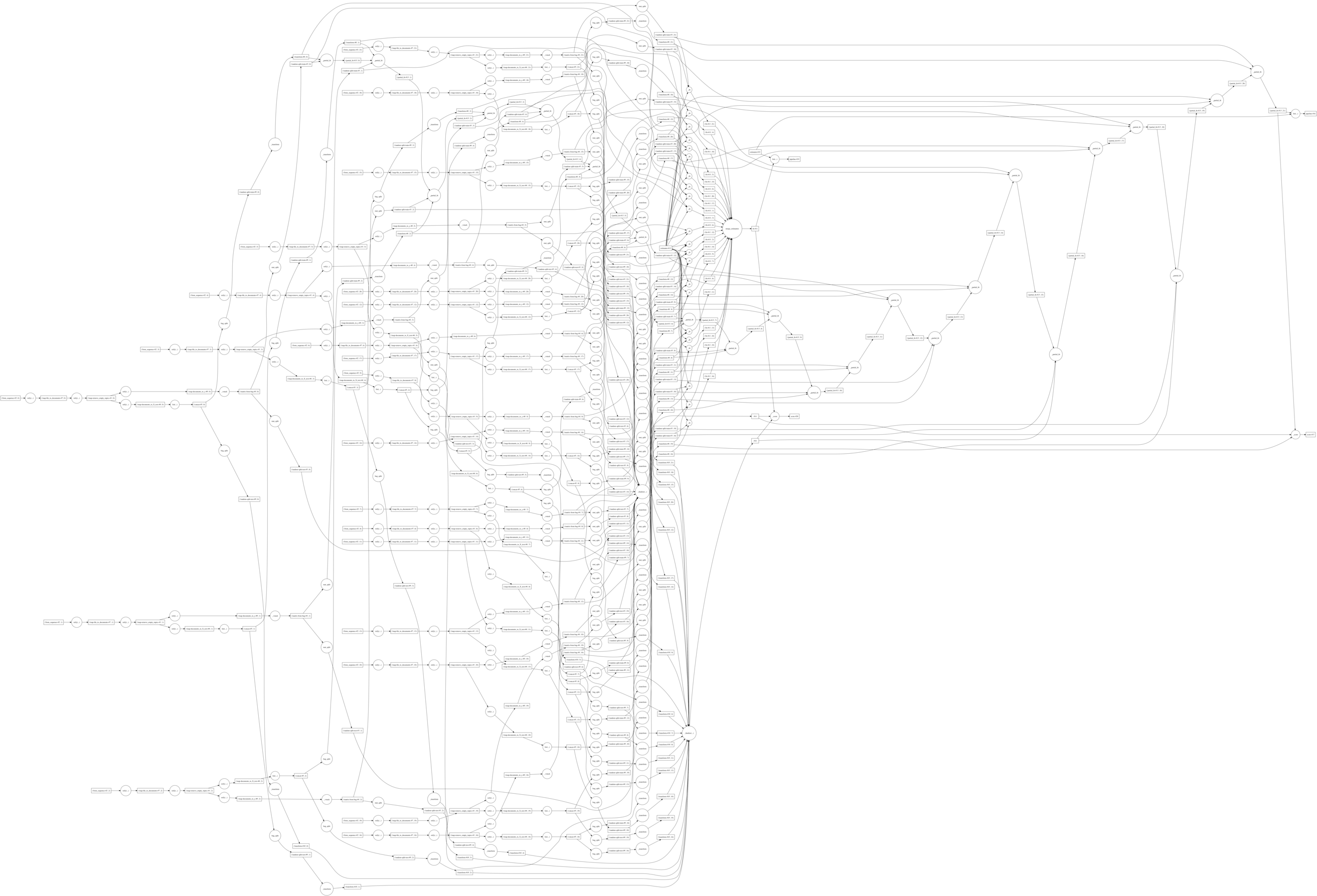
visualize([prof, rprof])

Looking at the above profiling plot, we can observe a few things:

• I'm able to achieve between 400 - 800% cpu usage. My machine has 4 real cores (8 virtual cores) so this is pretty optimal. Since we're only using 4 processes, the spikes to 800% are due to internal threading in certain scikit-learn operations.

• The dark blue rectangles are the disk reads and initial preprocessing steps. These are by far the most expensive parts of the computation. The overall profiling plot shows a nice structure of alternating reads and computations, which matches our expectations of streaming the data through memory.

What worked well

• The parallelization patterns are intuitive to use, and work with any estimator that matches the assumptions made. This means we don't need to create a new class for each scikit-learn estimator (there are a lot of them!).

• Because each estimator is lazy, we can fit several different estimators on the same data, but reuse intermediates results from each. This is more efficient.

• Since the wrapper classes implement the common fit, predict, score interface, they can be dropped into things like GridSearchCV, and everything should just work. This means we can do grid search and cross validation on out-of-core datasets (something we'll look at more in depth in the next post).

What could be better

• It's not clear that averaging coefficients is the best way for most estimators. In particular, I'm not sure what the behavior should be when all classes aren't present in all partitions.

• The approaches here are naive. This isn't necessarily a bad thing as it makes the library very easy to maintain. However, there are almost certainly more efficient/correct methods that could be used.

Help

I am not a machine learning expert. Is any of this useful? Do you have suggestions for improvements (or better yet PRs for improvements :))? Please feel free to reach out in the comments below, or on github.

This work is supported by Continuum Analytics and the XDATA program as part of the Blaze Project.